Back in 2013 John Gagnon wrote a very popular post detailing some of his favourite Excel tips and tricks.
We thought we’d update the list of classic shortcuts with a few that reflect some new functionality in Excel 2016.
New Excel tips for 2016:
1. Navigate ‘The Ribbon’ with ALT
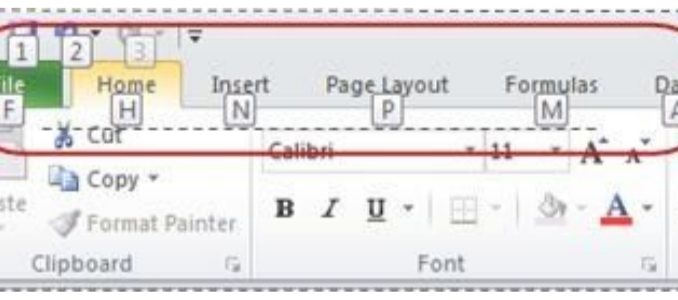
In Excel 2016 the ribbon refers to the menu of tabs (File, Home, etc.) at the top of your workbook. Simply hitting ALT will quickly highlight the related keys then used to jump to certain ribbon tabs.
For instance, ALT followed by M will take you to the ‘Formulas’ tab.
You can easily move between tabs by pressing ALT and using the left and right arrow keys, while CTRL + F1 toggles between hiding and showing the ribbon altogether.
2. Tell me what you want to do
Excel 2016 comes with a new helpful feature located in the ribbon, the ‘Tell me what you want to do’ search box.
Click the box, or if you are using Excel without a mouse hit ALT + Q to jump right to it. Whether it’s adding rows or using VLOOKUP, the box is very useful for new and old Excel users alike.
3. New Excel Tip: smart lookup
If you want information from beyond the realms of Excel, another new function for 2016 is the ‘Smart Lookup’ tool which allows you to make a Bing-powered internet search without leaving the Excel pane.
Smart Lookup is located in the ‘Review’ tab and can also be accessed by ALT + R + S.
Classic Excel tips:
Courtesy of John Gagnon. The following tips are accurate and still work as of September 2016.
4. Automatically SUM() with ALT + =
Quickly add an entire column or row by clicking in the first empty cell in the column. Then enter ALT + ‘=’ (equals key) to add up the numbers in every cell above.
5. Logic for number formatting keyboard shortcuts
At times keyboard shortcuts in Excel seem random, but there is logic behind them. Let’s break an example down. To format a number as a currency the shortcut is CRTL + SHIFT + 4.
Both the SHIFT and 4 keys seem random, but they’re intentionally used because SHIFT + 4 is the dollar sign ($). Therefore if we want to format as a currency, it’s simply: CTRL + ‘$’ (where the dollar sign is SHIFT + 4). The same is true for formatting a number as a percent.
6. Display formulas with CTRL + `
When you’re troubleshooting misbehaving numbers first look at the formulas. Display the formula used in a cell by hitting just two keys: Ctrl + ` (known as the acute accent key) – this key is furthest to the left on the row with the number keys. When shifted it is the tilde (~).
7. Jump to the start or end of a column keyboard shortcut
You are thousands of rows deep into your data set and need to get to the first or last cell. Scrolling is OK but the quickest way is to use the keyboard shortcut CTRL + ↑ to jump to the top cell, or CTRL + ↓ to drop to the last cell before an empty cell.
When you combine this shortcut with the SHIFT key, you’ll select a continuous block of cells from your original starting point.
8. Repeat a formula to multiple cells
Never type out the same formula over and over in new cells again. This trick populates all of the cells in a column with the same formula, but adjusts to use the data specific to each row.
Create the formula you need in the first cell. Then move your cursor to the lower right corner of that cell and, when it turns into a plus sign, double click to copy that formula into the rest of the cells in that column. Each cell in the column will show the results of the formula using the data in that row.
9. Add or delete columns keyboard shortcut
Managing columns and rows in your spreadsheet is an all-day task. Whether adding or deleting, you can save a little time when you use this keyboard shortcut. CTRL + ‘-‘ (minus key) will delete the column your cursor is in and CTRL + SHIFT + ‘=’ (equal key) will add a new column. From an earlier tip, think about CTRL + ‘+’ (plus sign).
10. Adjust width of one or multiple columns
It’s easy to adjust a column to the width of its content and get rid of those useless ##### entries. Click on the column’s header, move your cursor to the right side of the header and double click when it turns into a plus sign.
11. Copy a pattern of numbers or even dates
Another amazing feature built into Excel is its ability to recognize a pattern in your data, and allow you to automatically copy it to other cells.
Simply enter information in two rows which establish the pattern, highlight those rows and drag down for as many cells as you want to populate. This works with numbers, days of the week or months!
12. Tab between worksheets
Jumping from worksheet to worksheet doesn’t mean you have to move your hand off the keyboard with this cool shortcut. To change to the next worksheet to the right enter CTRL + PGDN. And conversely change to the worksheet to the left by entering CTRL + PGUP.
13. Double click format painter shortcut
Format Painter is a great tool which lets you duplicate a format in other cells with no more effort than a mouse click. Many Excel users (Outlook, Word and PowerPoint too) use this handy feature, but did you know you can double-click Format Painter to copy the format into multiple cells? It’s quite a time-saver.
Source: ClickZ
Link: 13 time-saving Excel shortcuts & tips for marketers


Leave a Reply